Building Bridges with the Area Model: From Multiplication to Algebra

A Planned and Purposeful Journey of Multiplication (and Beyond!)

Do your students have a consistent journey in multiplication? Or do they learn method after method without meaning but simply process.

If you consider multiplication from early multiplication to factorising double brackets, maybe you are teaching 8 different methods of multiplication?

What if we could use one model and then compare and contrast the changes to that model at each point.

This is my reflections on what building a continuous planned and purpose journey of multiplication can look like.

Table of Contents

Laying the Foundation

• From Arrays to Area

• Visualising the Commutative Law

• Scaled Multiplication Table

Expanding the Model

• Multi-digit Multiplication

• Distributive Law in action

• Expanding brackets

Extending the Model

• Factorisation

• Completing the Square

• Polynomial Division

The Plenary

Laying the Foundation: The Area Model in Early Multiplication

From Arrays to Area:

The journey begins with students' initial introduction to multiplication. We leverage the area model by connecting multiplication to the concept of area using arrays. This early connection, potentially as early as ages 4 or 5, is crucial. Students can see the different shapes, use different items before building with multilink cubes and counting squares within rectangles, establishing a link between spatial awareness and numerical understanding. Number blocks provides an excellent introduction to arrays and making the link to times tables.

Visualising the Commutative Law:

This stage allows for a visual and intuitive grasp of the commutative law. Students see that a 3 × 4 array occupies the same space as a 4 × 3 array, leading to the understanding that 3 × 4 = 4 × 3. The use of blocks (shown below) can reinforce this, embedding the area concept within our base-ten system and preparing students for volume models later on.

Scaling Up: Multiplication Tables and the Times Table Square:

We can represent multiplication tables as scaled area models. Constructing a times table square visually makes the link to the earlier arrays. highlights square numbers along the leading diagonal. The symmetry across this diagonal provides a further compelling visual demonstration of the commutative law. One that students are able to see for themselves.

Expanding the Model: Multi-Digit Multiplication and Algebraic Connections

Extending to Multi-Digit Multiplication:

As learners progress to multiplying larger, multi-digit numbers, the area model evolves to incorporate place value. While it can certainly be used as a method for calculation, the emphasis here is on reinforcing the significance of place value referring back to what they have done before to take the next steps on their planned and purposeful journey.

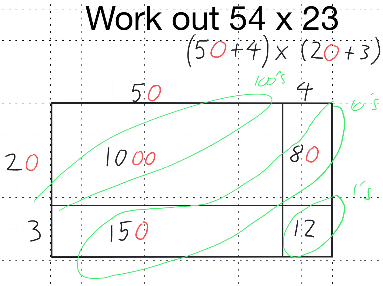
For example, 54 × 23, first, we partition the numbers as (50 + 4) × (20 + 3), creating the grid for our area model:

In my previous post I mentioned how historically I stopped using ‘grid method’. A key difference I see is that the rebranding of the area model means that this is not simply a method for students to arrive at the correct answer; it has a deeper, connected layer. Firstly, we are finding the area of a rectangle by dividing it up into its parts. This was never something I connected with when I used the ‘grid method’. Secondly, I have tried to convey with colour coding. There is place value running through the diagonals in the area model. So let’s discuss this a little more.

Here, in the top left-hand corner, we explicitly discuss that multiplying 5 tens by 2 tens results in 10 hundreds (1000), above I have used red to denote place holders. Similarly, 4 ones multiplied by 2 tens gives 8 tens (80), 5 tens multiplied by 3 ones gives us 15 tens (150), and finally, 4 ones times 3 ones equals 12 ones. Over time I will look to build on and highlight these features to students.

Previously I would have then laid out a large column addition to the right hand side. What I tend to do now is to sum the diagonals. Why, firstly this reinforces and interleaves our understanding of place value secondly because this foreshadows the work I do later with expanding and factorising brackets.

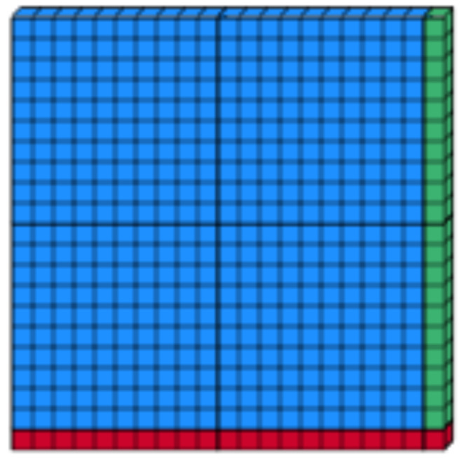
Earlier in a student’s journey we can illustrate this visually using base-ten manipulatives initially, then transition to the abstract or semi abstract representation of the area model. The diagram below shows how 54 × 23 can be represented using base-ten.

By highlighting the diagonals within the area model grouping the place value. This understanding could then provide a natural bridge to an efficient methods like lattice multiplication, offering a strong conceptual foundation rather than a rote procedure. As shown we can use this area model to move through a progression: from concrete manipulatives to visual representations with varying layers of abstraction. I quite like having my internal rectangles as being different sizes to give the visual cue that these numbers have different orders of magnitude.

Building Fluency with the Distributive Law:

The power of the area model extends beyond just base-ten partitioning. By exploring alternative ways to partition numbers, we can build a robust conceptual understanding of the distributive law.

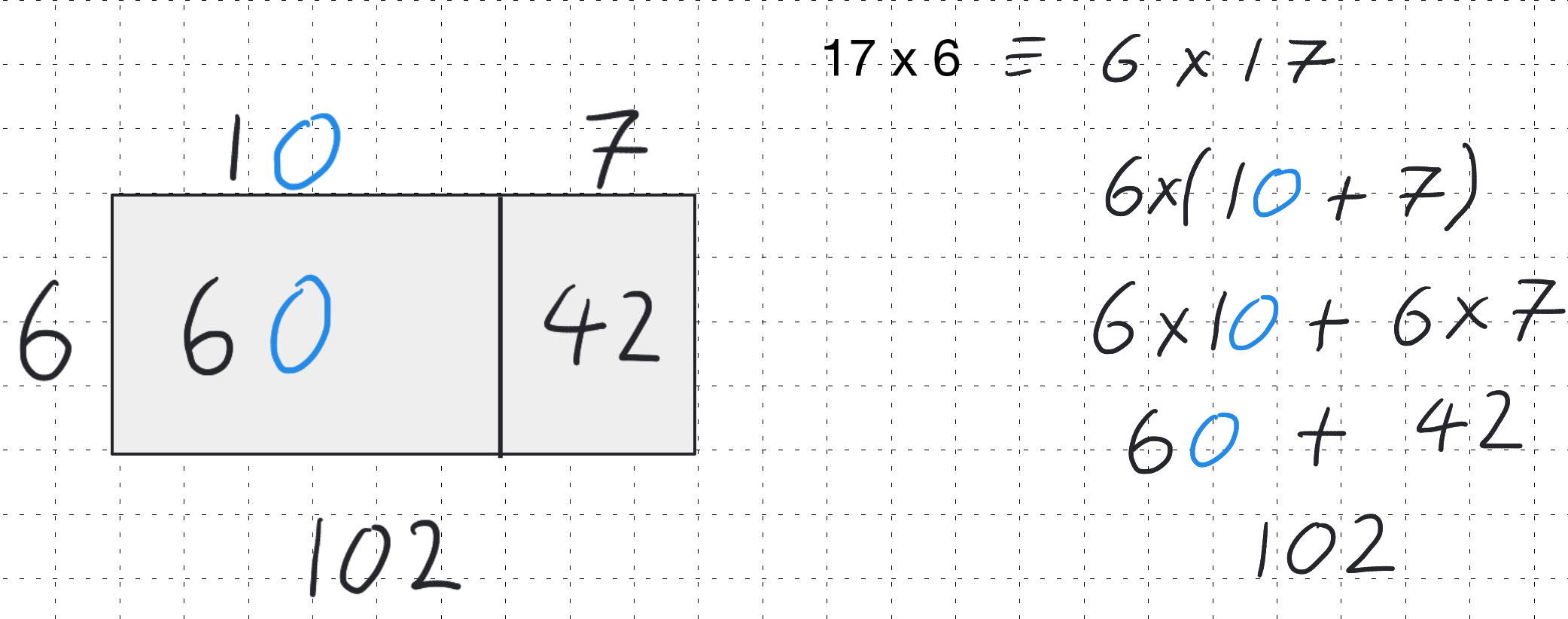
For instance, we might explore 17 × 6 as (10 + 7) × 6 or even (20 - 3) × 6:

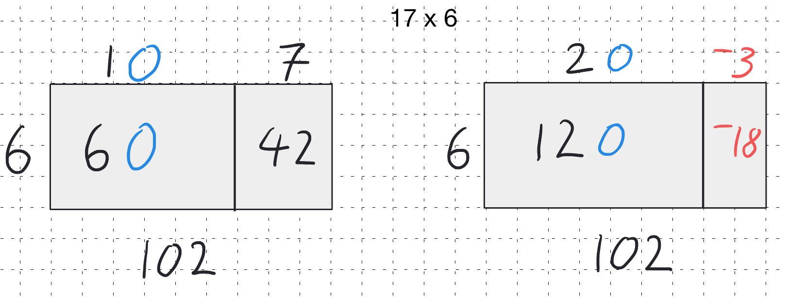
The area model naturally lends itself to implicitly using the distributive law of arithmetic. We could choose to have the area model alongside the written working this can be seen below.

This highlights how the area model can also be applied to develop a deep understanding of the underlying mathematical structure.

A really intriguing example when choosing or question set - if we have secured students understanding of directed number - we can build in difference of two squares questions, such as 21 × 19. We should set the partition of these numbers up for our students as (20 + 1) × (20 - 1):

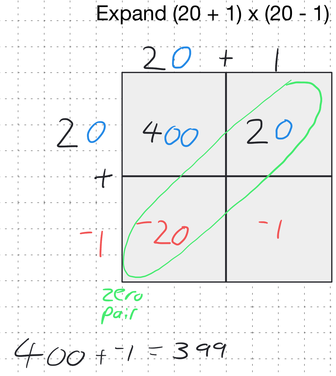
Notice here how the terms along the diagonal involving the tens (20 × -1 = -20 and 1 × 20 = 20) create a "zero pair" when combined. Visually, we can see these ten terms summing to zero. This is particularly powerful if you have used tiles or two sided counters previously. Using mathsbot we can create negated base-ten and see this zero pair as below.

This not only provides us with a deeper connection and varied practise for partitioning numbers differently but also offers a visual and conceptual link to the algebraic identity:

\((a+b)(a-b)\equiv a^2-b^2\)

The difference of two squares can be introduced and foreshadowed before students formally encounter the algebraic identity shown above.

Transitioning to Algebraic Multiplication: Expanding Brackets

This solid foundation in numeric work with the area model then seamlessly transitions to the algebraic realm, where we encounter multiplication involving an unknown base, represented by a variable.

Consider the multiplication of (5x + 4) × (2x + 3). We can directly compare this to the earlier numeric example of 54 × 23, explicitly partitioning it as (50 + 4) × (20 + 3). By placing these two side-by-side, we can encourage students to identify similarities and differences.

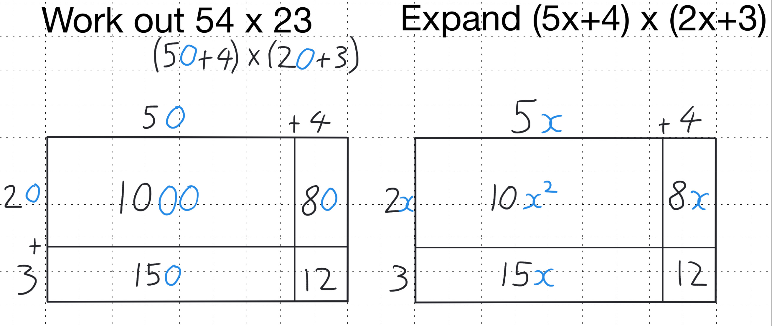
Students will often readily observe that the zeros in the numeric example have been "replaced" by x's in the algebraic one. This opens up rich discussions about the concept of a base – where 10 is our familiar base, and x represents an unknown base. We can pose questions about substitution: "What would the value of x need to be for both expressions to yield the same numerical result?" This fosters deep connections between the numeric and algebraic, encouraging genuine mathematical thinking. Students are making relatively simple observations that hint at profound mathematical relationships.

If we are using manipulatives to support the model we could also utilise our base-ten again here, but now run a comparison between base-ten and algebra tiles.

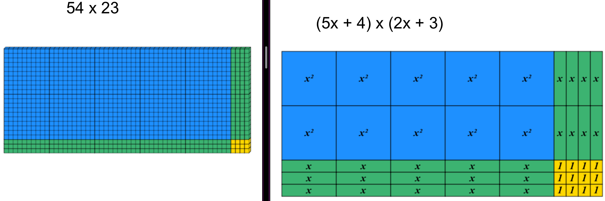
At this points the diagrams are incredibly close. It is only the length of the 10 being replaced by an unknown length. Even the colour coding is the same.

Extending the Model: Factorisation and Completing the Square

Factorisation as the Reverse Journey:

Typically a variety of methods maybe used to factorise each different from the last. Some might be tempted to fall into methods which break down such as FOIL. Maybe we think that catchy phrases will students understanding such as crab claw or homers hair. However, the area model provides an intuitive pathway to factorisation.

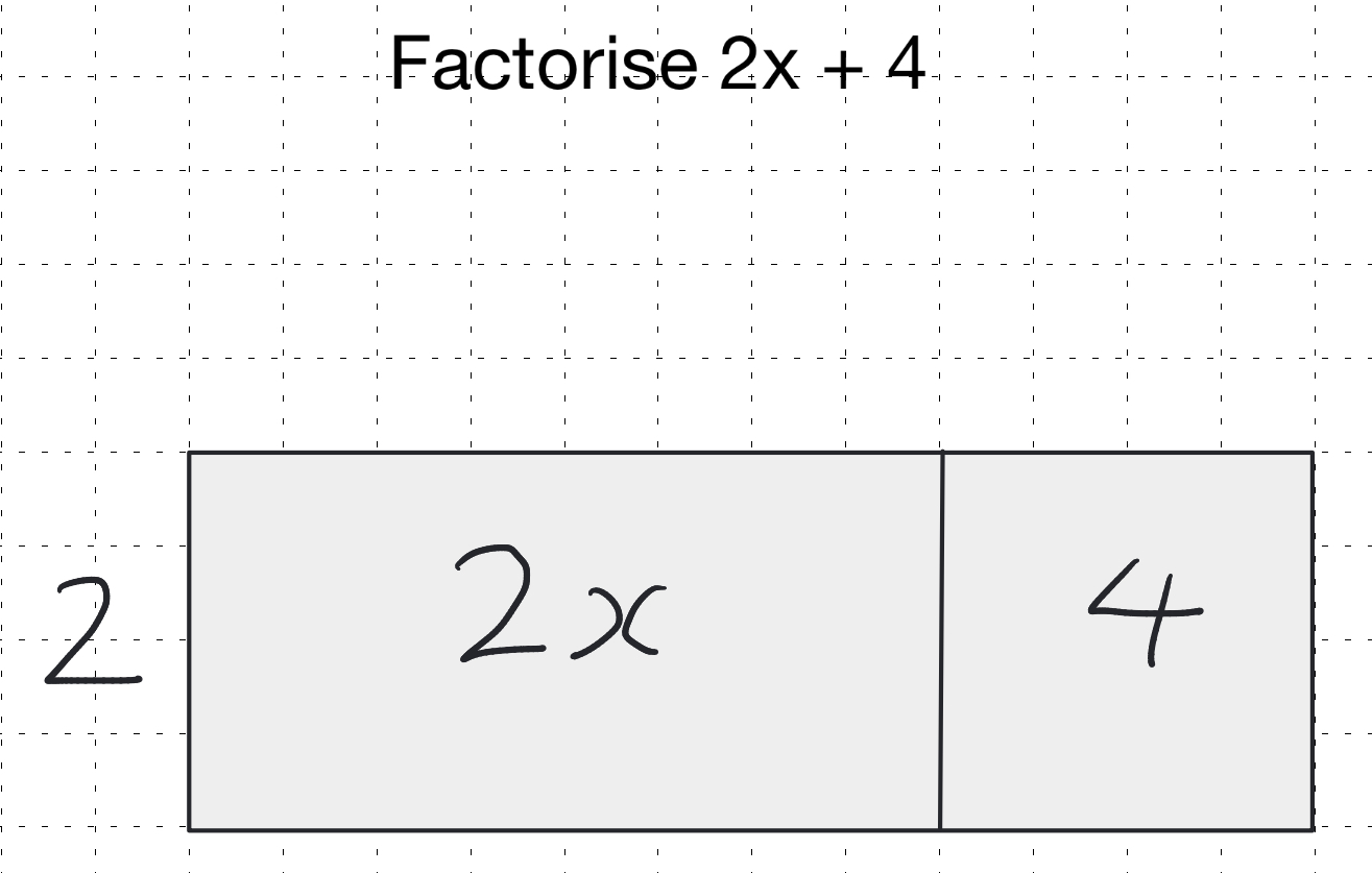
We can start by factorising into single brackets. This can be introduced in a really simple way by giving a partly factorised area model and asking students to complete the model.

After this we can use the idea of highest common factor to find the initial single starting factor. This can be particularly supported if we foreshadowed this factorising work with completing missing number numeric versions of the area model at an earlier stage. More on this later.

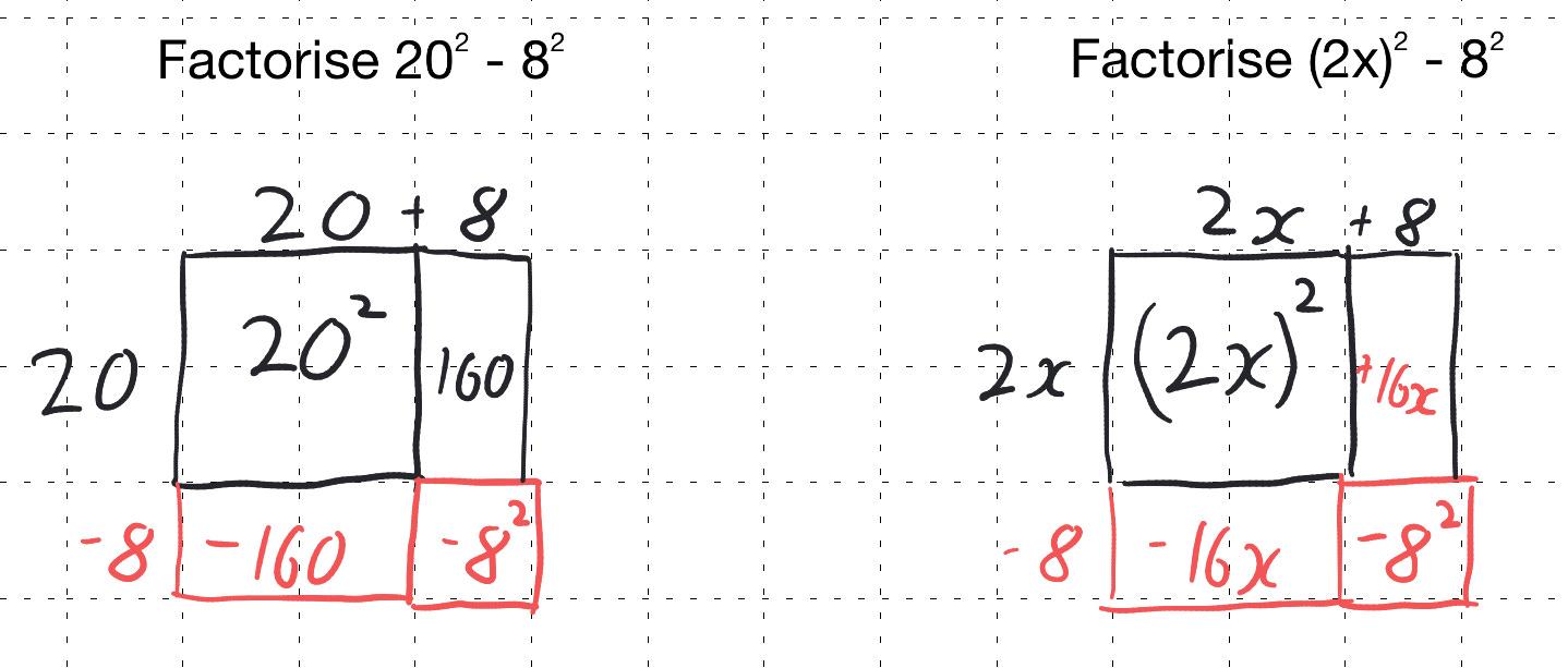
If we are using this highly visual approach and have explored 2 digit by 2 digit difference of two square. Our next step for factorising can be difference of two squares. This feels quite counter intuitive when you are used to factorising difference of two squares later, but the visual model enables this to happen numerically sooner that factorising into double brackets. Once students are competent numerically and with algebra tiles difference of two squares can be factorising algebraically.

Next we can consider factorising into double brackets. Having already recognised that the diagonals represent terms with the same place value (or the same power of x), we can now reverse the process. When factorising a quadratic expression like 2x² + 7x + 3, we aim to find the dimensions of the rectangle that would give us this area. The "puzzle-like" nature of fitting the terms into the grid, often guided by the sum of the 'middle' terms along the diagonal, makes factorisation a more visual and less abstract process.

As mentioned earlier, this led me to consider its application purely within the numeric domain. I discovered that I could create "missing number" puzzles using the area model, where students would naturally employ factorising strategies to solve them, entirely divorced from algebra. For example:

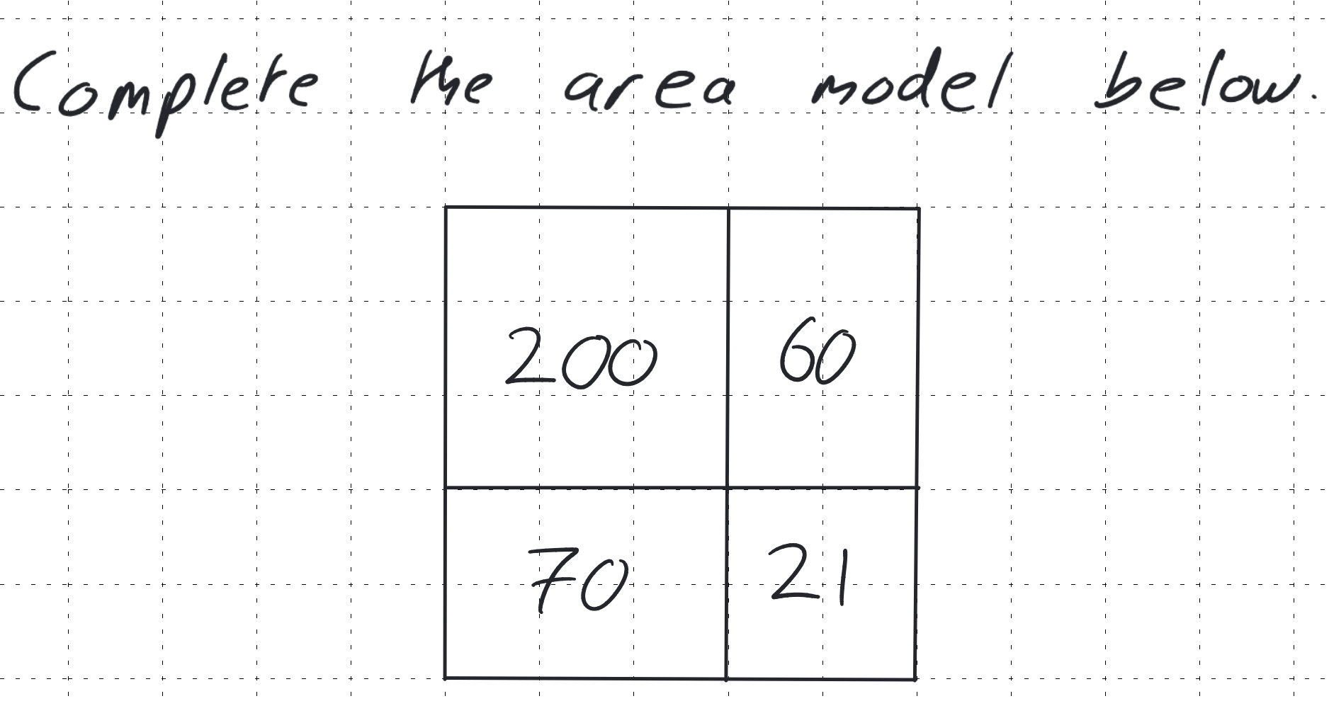
This reinforces the understanding that the lengths of the sides of the rectangle represent the factors of the total area – hence the term "factorising." It shifts the understanding away from simply viewing factorising as the inverse of expanding, providing a continuously developing schema.

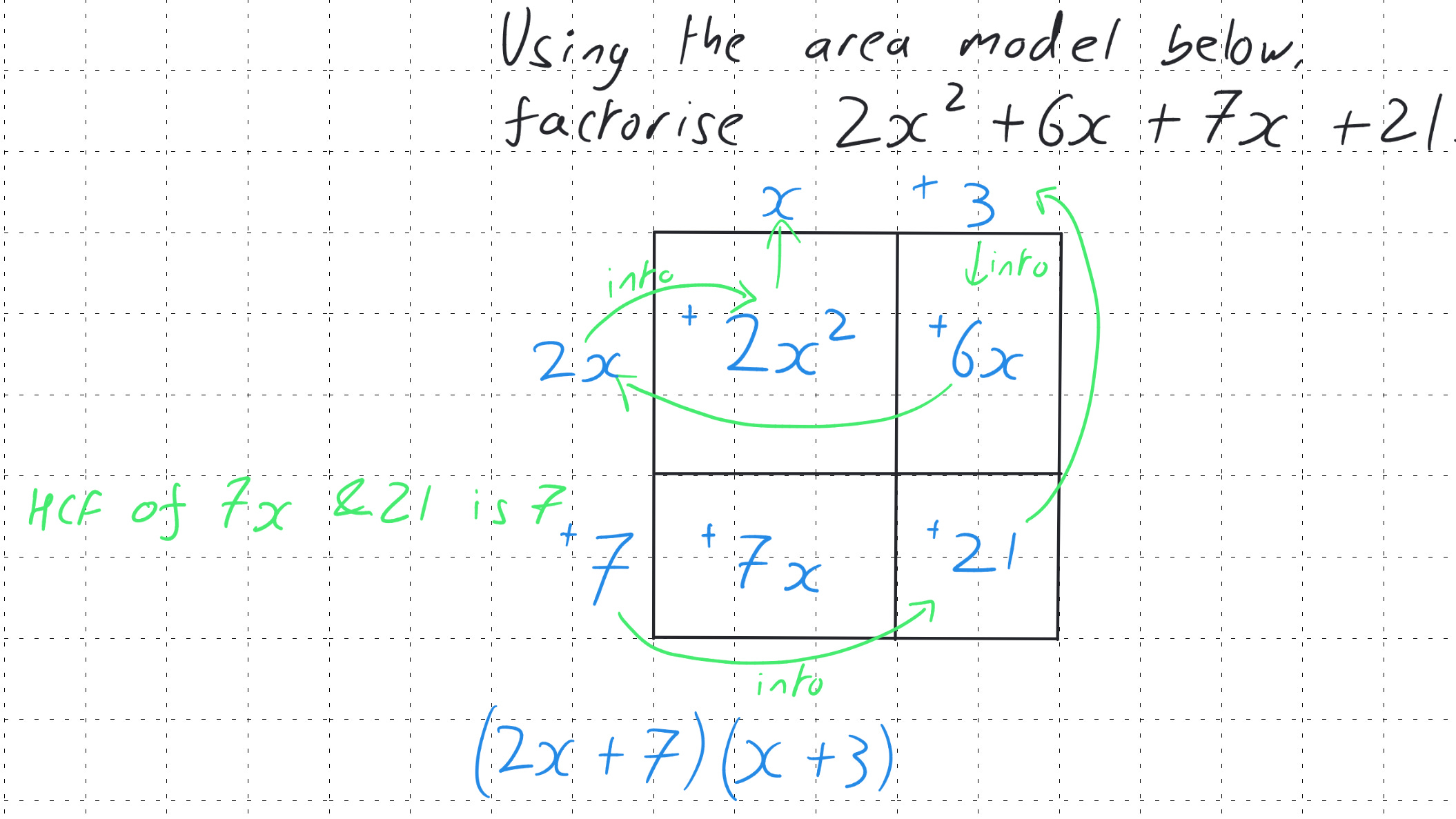
This can then lead us later onto be able to factorise 2x² + 6x + 7x + 21. As shown below. The green indicates explained not written working. You need to remember the quantity of work is that an example below is close to the culmination of at least 4 years of working with the same progressive area model.

Our final two steps for GCSE factorisation would be to have combined x terms, and to introduce ac. Combined x terms can be reinforced as the progression of the diagonals giving us our place value, ac is the one aspect that I tend to have to say you now need this step, please comment if you have a good approach to explain ac.

Completing the Square:

The versatility of the area model extends even further into the realm of completing the square. Consider a quadratic expression like x² + 6x. We can represent the x² term as a square with side length x, and the 6x term as a rectangle with one side x and the other side 6. To "complete the square," we aim to arrange these pieces into a larger, almost complete square.

If we take the 6x rectangle and divide it equally into two rectangles of size 3 × x, we can place one on each side of the x² square. This forms an 'L' shape. To complete the square, we need to fill the missing corner. The dimensions of this missing square would be 3 × 3 = 9.

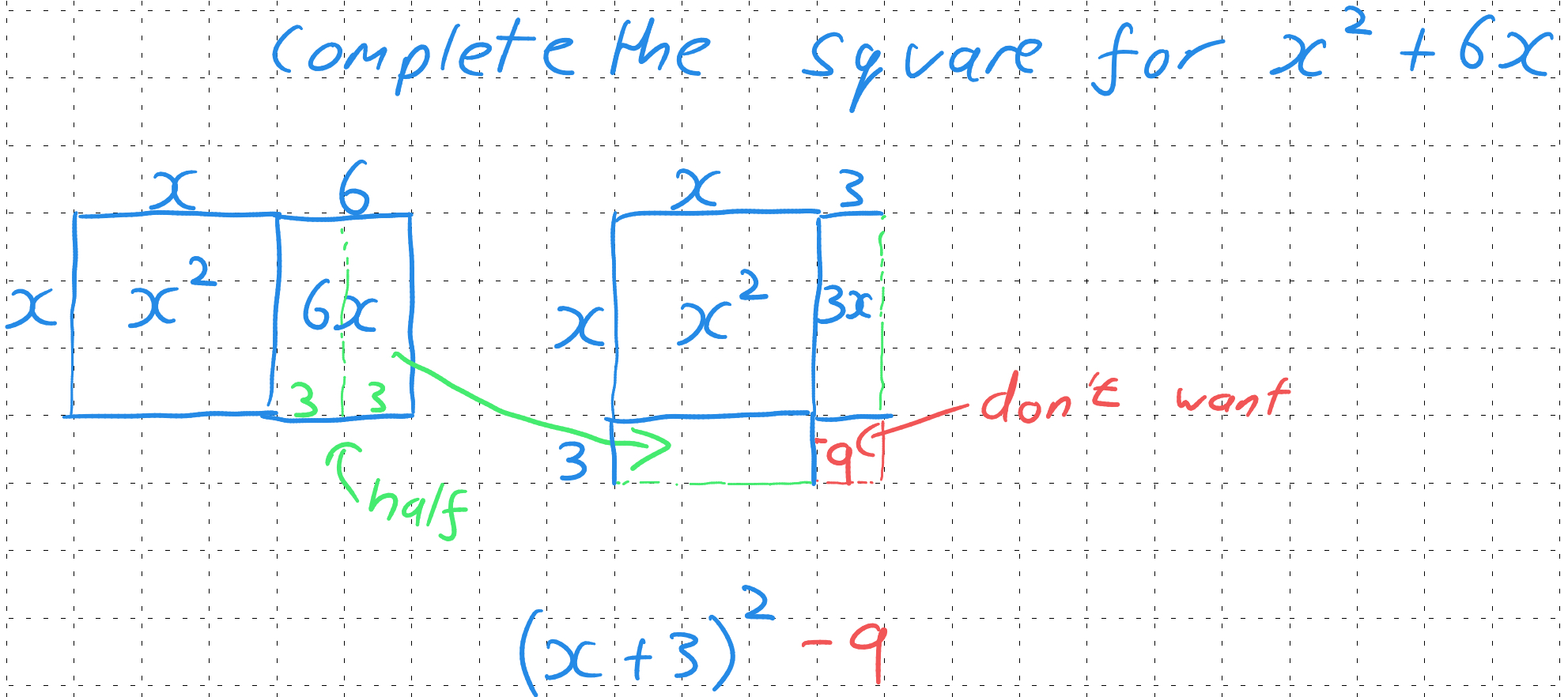
Thus, x² + 6x can be seen as part of the larger square (x + 3)², however it generates this additional area of 9 which we need to subtract. Therefore, x² + 6x = (x + 3)² - 9.

This visual manipulation of the area model to complete the square provides a powerful connection to the algebraic process. Furthermore, it lays the groundwork for understanding the graphical representation of quadratic functions. The completed square form, (x + h)² + k, directly reveals the coordinates of the vertex of the parabola (-h, k). In our example, the vertex of y = x² + 6x would correspond to the shift implied by (x + 3)² - 9, giving a vertex at (-3, -9). The area model provides a tangible link between the algebraic manipulation and the key features of the graph which in turn can be connected to graph transformations. This progression can help to highlight the interconnectedness of mathematics.

Moving beyond GCSE: Division of polynomials.

While the above is an impressive journey through maths, I really like my final exploration in maths. We are going to be working out the following:

\((x^3+18x^2+105x+196)\div(x+4)\)

In case readers aren’t aware first let’s discuss the traditional method to approach this is algebraic long division. This approach is shown below;

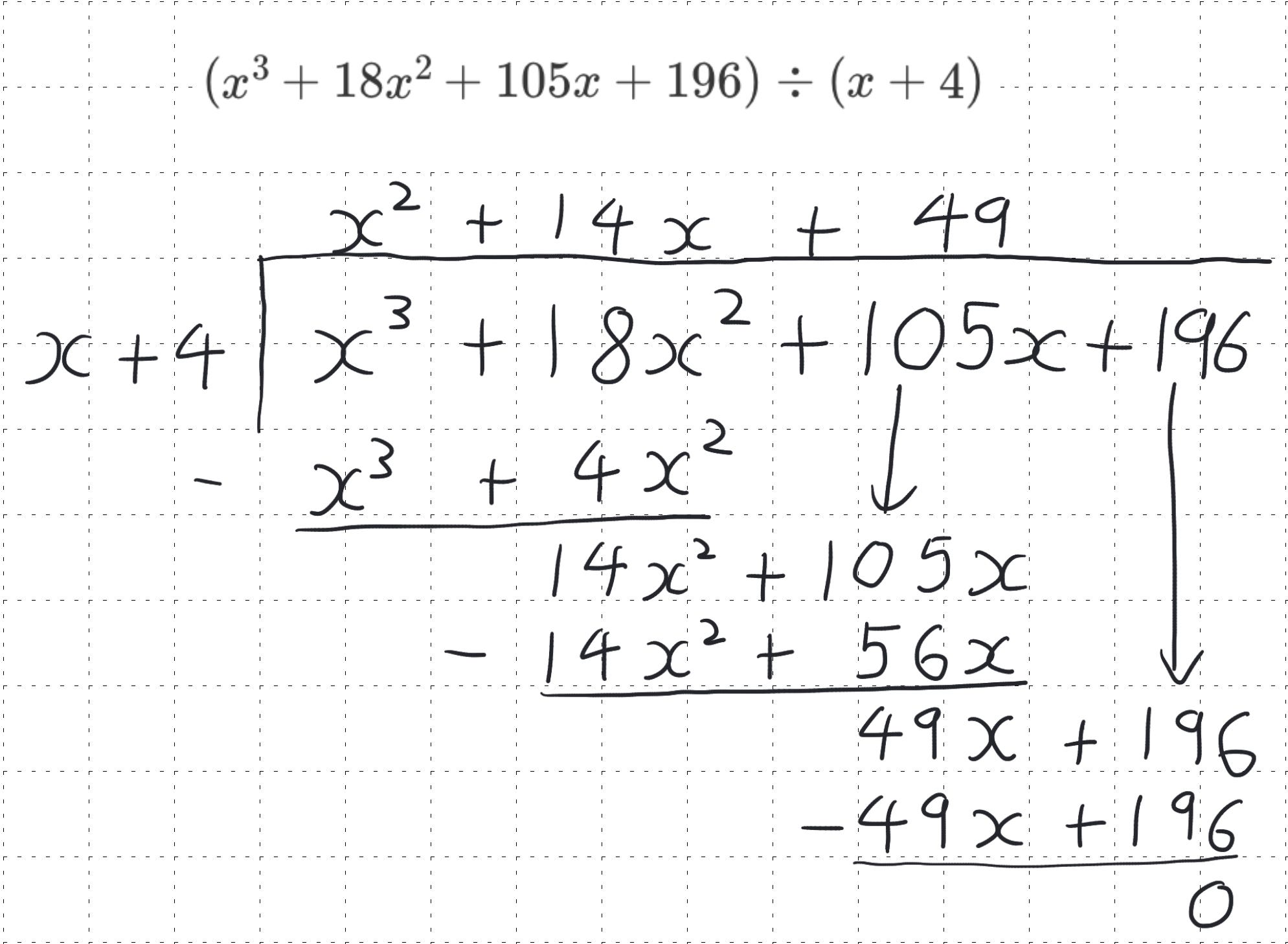
The way in which it works follows the approach of normal long division quite closely so works quite well as a progressive coherent approach, but, that’s part of the problem. Very students now learn formal long division; compressed division or “bus stop” has become the prevalent approach. Which means that to teach algebraic long division well, you first need to teach a new division approach. This undermines the whole approach of trying to build a coherent approach.

So let’s see how this looks using the area model instead;

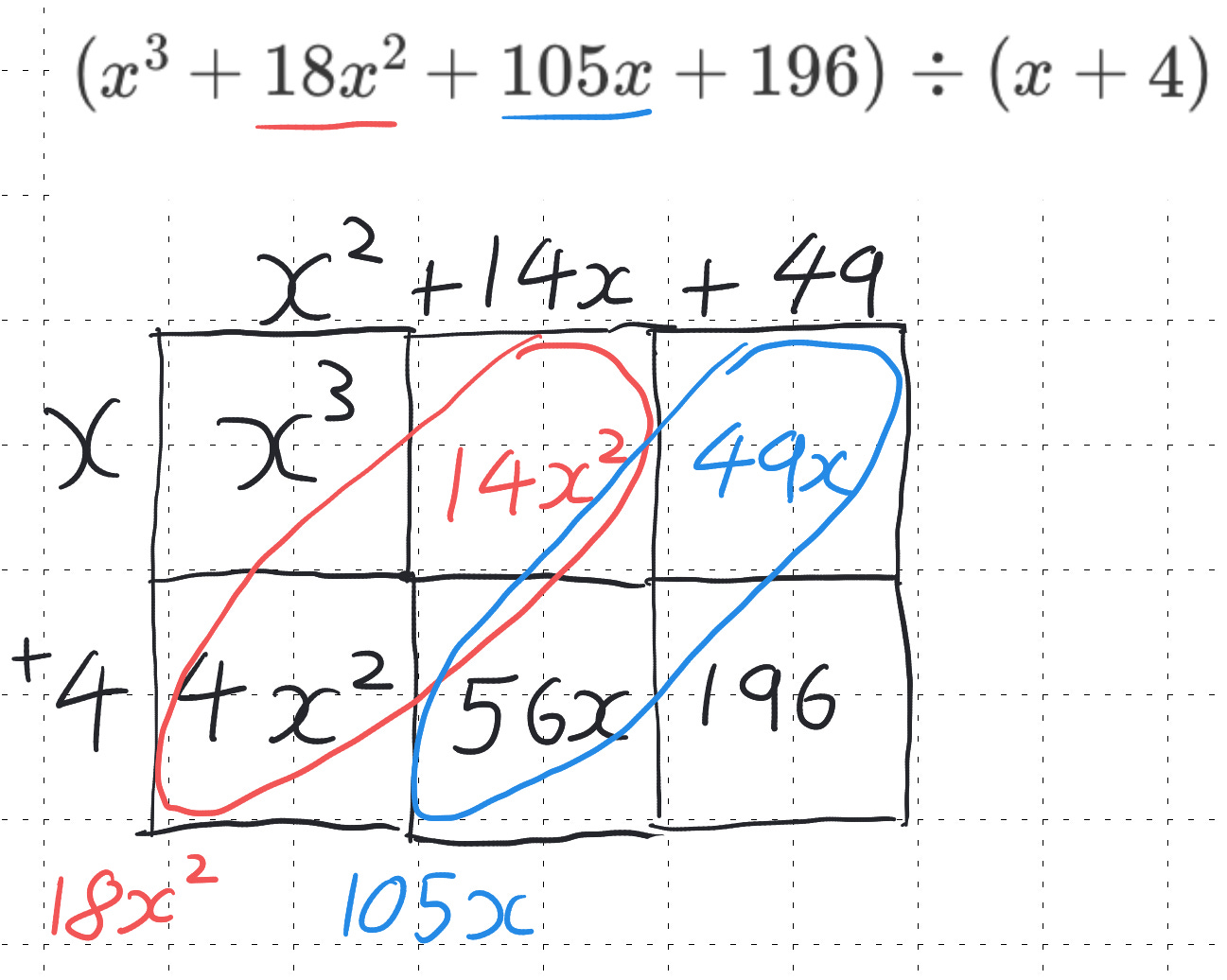
What is fantastic about this approaches is it pulls in some of our early multiplication ideas that we may have highlighted that the diagonals have this place value concept running through them. Now we are using them as a reverse of that earlier idea. It’s an idea that we used within factorising quadratics that the x’s summed along the diagonal. Now we are using this for different powers of x. There are no particularly new concepts if the progression has been followed, just modified application.

The Plenary of: A Planned and Purposeful Journey of Multiplication

By consistently using the area model, supported by manipulatives like algebra tiles, we can create a truly planned and purposeful journey through multiplication and into more advanced algebraic concepts like completing the square and its graphical implications. The method is progressive, the deeper you go the more it fosters a deeper, connected understanding, empowering students to see the underlying structure and beauty of mathematics. This is a broad overview of a planned coherent journey, but there are so many areas still left to discuss for example we haven’t considered decimals or fractions. There are still so many places we can go deeper

---

Acknowledgments

The images of Dienes/base-ten blocks and algebra tiles have been created using the mathsbot.com website.

The idea’s here are a culmination of both my own throughts and reflections as well as the various books, podcasts, webinars and conferences that I have read, watched and listened to over the last couple of years as well asthis includes: Visible Maths, Teaching for Mastery, Mr Barton’s Maths Podcast, Beyond Good, MathsConf online, Complete Maths CPD events amongst others. I have aimed to put my own thoughts into this process and not directly aimed to copy any other work but will have been influenced by others.